A Predictive Framework for Forecasting Soccer Match Outcomes by Analyzing the Goal Count Achieved by A Specific Team
|
[1] Universidad de Teesside – Inglaterra, evelynparker3339@gmail.com, https://orcid.org/0009-0006-2181-1701
|
|
|
|
Copyright: © 2023 by the authors. This article is an open access article distributed under the terms and conditions of the Creative Commons
Received: 18 September, 2023
Accepted for publication: 02 November, 2023
|
ABSTRACT Soccer, a widely embraced sport, proves to be an intriguing subject for study due to its substantial data output. This article introduces a machine learning-based model designed to predict the success or failure of a soccer team based on its goal-scoring performance. The model employs four machine learning classifiers: Linear Regression, Support Vector Machines, Naive Bayes, and Decision Trees. Drawing on data from the Mexican football league spanning from 2012 to March 2020, the study is bifurcated into two segments: one encompassing draws and the other excluding them, aimed at unveiling the impact of draws on the analysis. The proposed model achieved an accuracy ranging from 81% to 84% when draws were excluded, while incorporating draws resulted in an accuracy range of 72% to 75%.
Keywords: Soccer; Machine Learning; Predictive Model
|
||
Un Marco Predictivo para Pronosticar los Resultados de Partidos de Fútbol Analizando la Cantidad de Goles Logrados por un Equipo Específico
RESUMEN
El fútbol, un deporte ampliamente aceptado, resulta ser un tema intrigante para el estudio debido a su generación significativa de datos. Este artículo presenta un modelo basado en aprendizaje automático diseñado para predecir el éxito o fracaso de un equipo de fútbol basado en su rendimiento en la marcación de goles. El modelo utiliza cuatro clasificadores de aprendizaje automático: Regresión Lineal, Máquinas de Soporte Vectorial, Naive Bayes y Árboles de Decisión. Basándose en datos de la liga de fútbol mexicana desde 2012 hasta marzo de 2020, el estudio se divide en dos segmentos: uno que incluye empates y otro que los excluye, con el objetivo de revelar el impacto de los empates en el análisis. El modelo propuesto logró una precisión que oscila entre el 81% y el 84% al excluir los empates, mientras que la inclusión de los mismos resultó en un rango de precisión del 72% al 75%.
Palabras clave: Fútbol; Aprendizaje Automático; Modelo Predictivo
INTRODUCTION
Soccer, the globally beloved sport, experienced a temporary suspension starting from March 2020 due to the pandemic. The conventional methods of prediction, relying on domain expert forecasts and statistical approaches, face challenges with the growing volume of diverse football-related data [1]. Machine Learning, a subset of Artificial Intelligence, addresses this challenge by exploring methods for pattern recognition in datasets undergoing analysis. It involves the development of algorithms capable of learning from data and making predictions or regressions, with each methodology hinging on constructing a specific model [11].
During the learning phase, data subjected to pattern recognition can consist of arrays with a single value per element or multivariate values, often referred to as characteristics or attributes [11]. Machine learning is categorized into three main areas: supervised, unsupervised, and reinforcement learning. Given our focus on prediction based on known properties learned from training data, our approach centers around supervised learning. In this context, the dataset includes both inputs (feature set) and desired outputs (objectives), enabling us to understand the data properties and make predictions [5].
The capability to monitor algorithm training significantly contributes to the widespread adoption of machine learning. This paper proposes the creation of a supervised learning model utilizing various machine learning algorithms such as Logistic Regression, Support Vector Machines, Decision Trees, and Naive Bayes. The aim is to predict the outcome (winner or loser) of a football team based on the number of goals scored in a match, without consulting the goals scored by the opponent team. The dataset is prepared from information provided by a betting support page, consolidating results from the first division of the Mexican football league spanning the 2012 season to March 2020 [1].
Related Work
In [2], Deep neural networks (DNNs) and artificial neural networks (ANNs) have been used to predict the results of football matches, using a data set that collects the results and performances of international football teams in previous matches, where they divide the data sets into sections for training, validation and testing, they used their model to predict the results in the 2018 World Cup, obtaining an accuracy of 63.3 %. In [3], the authors use the APSO automatic clustering method to divide the data set, in this case professional soccer players, into their position: goalkeepers, midfielders, defenders and strikers, in addition to applying a combination of machine learning techniques of particle swarm optimization (PSO) and support vector regression (SVR), to estimate the value of football team players in the transfer market, where they achieve an accuracy of 74 %. 1 https://www.football-data.co.uk/mexico.php In [4], the authors propose a Softmax regression model, which is a generalization of the logistic regression model, to predict the outcome of football matches based on the publicly available information of results of previous matches, of the Portuguese first division league. The prediction is formulated as a problem of classification with three classes: victory of the home team, draw or victory of the visiting team (Away Team).
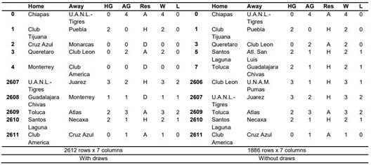
Table 1. Initial dataset
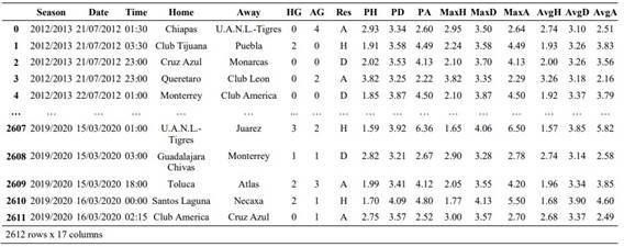
METHODOLOGY
Drawing inspiration from [5], our proposed model involves an initial step of dividing the data into two sets: a Training set and a Testing set. This diverges from the approach in [5], where all data is utilized. In addition to Logistic Regression, we employ various supervised learning algorithms, including Naive Bayes, Decision Trees, and Support Vector Machines. This diverse application aims to compare results and enhance overall accuracy. To optimize efficiency, our analysis is conducted first considering draws and then excluding them.
Dataset Acquisition
The dataset for this study is sourced from the aforementioned page, encompassing match results from the Mexican soccer league teams during the seasons spanning from 2012 to March 2020. The dataset comprises results from 2,612 games in the first division of the Mexican soccer league, featuring 17 characteristics for each match, such as season, date, match time, home and visiting teams, goals scored by each team, match winner, and percentage data (refer to Table 1).
Data Exploration and Inspection
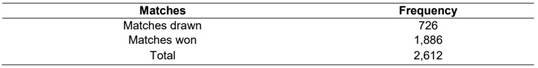
Upon scrutinizing the dataset, we identify that out of the 2,612 matches played, 726 resulted in draws. Consequently, the dataset excluding draws is reduced to 1,886 instances where one team emerged victorious, leading to the other's defeat. Table 2 illustrates that draw matches constitute 27.7% of the total matches played. This study predominantly focuses on the number of goals influencing a soccer team's victory or defeat, as depicted in Figure 1. The analysis indicates that with zero or one goal, losing is more probable, whereas with two or more goals, the likelihood of winning a match increases.
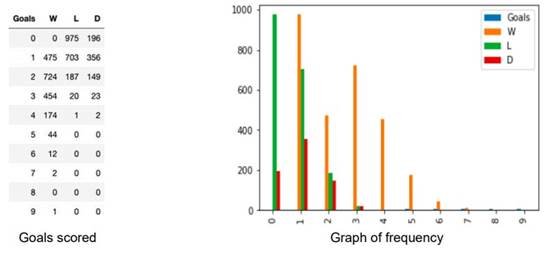
Figure 1: Distribution of Goals and Frequency
Table 2: Summary of Drawn and Won Matches
Data Preprocessing
In the context of this study, aimed at predicting the outcome (winner or loser) based on team goal counts, the information contained in the following columns suffices:
- HG: Number of goals scored by the home team.
- AG: Number of goals scored by the visiting team.
- Res: Result of the game, where:
Ø H: The local team wins.
Ø A: The visiting team wins.
Ø D: Draw.
Table 3 displays the dataset with the relevant columns.
Feature Extraction
To enhance the set of features, two additional columns are introduced into the table:
· W: Denoting a winner.
- L: Denoting a loser.
Table 3: Selected Columns in the Dataset
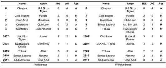
Table 4: Dataset with Additional Columns W and L
Columns W and L represent the number of goals determining whether a team won or lost the match, respectively. In instances of a draw (D), the values of W and L are identical, as observed in rows 2, 4, and 2608 of Table 4.
To construct the feature vector X, column W is concatenated with column L, forming a unified vector, as depicted in Figure 2. The feature vector X comprises 5224 data points derived from the teams' performance in the 2612 matches played when considering draws. The vector's size is reduced to 3772 when excluding draws. It's noteworthy that a team can secure a victory with two goals, as exemplified in the second match with a score of 2-0. Conversely, a team can also suffer a defeat by two goals, as illustrated in the antepenultimate match with a score of 3-2. Additionally, draws are accommodated, exemplified by the third match with a score of 0-0, where the score appears in both W and L.
Given that a team's outcome is determined by a specific number of goals, the label vector Y is generated from the feature vector X. In the label vector Y, the marker for the winning team is replaced by 1, while that for the losing team is replaced by 0, as illustrated in Figure 3.
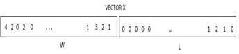
Figure 2: Vector X
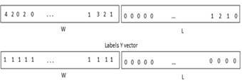
Figure 3: Feature and Label Vectors
Classification Model
In the realm of machine learning, a standard practice involves assessing an algorithm's performance. This evaluation entails dividing the data into two segments: a training set, where the algorithm learns the data properties, and a test set, used to validate those properties [5]. To create the training and test vectors, the X and Y vectors are partitioned in a manner that preserves 75% of the size for the training vector, while the remaining 25% constitutes the test vector. It's crucial to allocate a percentage of the data for model performance verification.
Following the selection of the training and test sets, we employ four machine learning algorithms for constructing the prediction model, encompassing Logistic Regression, Naive Bayes, Support Vector Machine, and Decision Trees.
Logistic Regression
Logistic regression serves as a statistical and probabilistic classification model designed for predicting a binary response, specifically the outcome of a categorical dependent variable (i.e., a label of class Y). This prediction is based on one or more variables comprising the feature vector X [5].
An exemplification of the logistic function is expressed as follows:

This function proves valuable as it confines the output to values ranging between 0 and 1, offering an interpretable representation akin to a probability.
Naïve Bayes
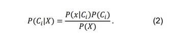
In the context of an n-dimensional vector, denoted as X = (x1, x2, x3, ..., xn), the Bayesian classifier allocates each X to one of the target classes within the set {C1, C2, ..., Cm}. This assignment hinges on the probability that X belongs to the target class Ci. In essence, X is assigned to class Ci if and only if the condition P(Ci | X) > P(Cj | X) holds true for every j within the range 1 ≤ j ≤ m. It is imperative to reserve a percentage of the data for verifying the model's functionality.
Following the selection of training and test sets, we employ four machine learning algorithms for constructing the prediction model, including Logistic Regression, Naive Bayes, Support Vector Machine, and Decision Trees.
P(Ci | X)> P (Cj | X) for every j such that 1 ≤ j ≤ m where:
To streamline computation, the Naive Bayes classifier is developed under the assumption of conditional class independence, signifying that attributes are considered independent for each class.
Support Vector Machine
Originally devised for fitting a linear boundary between samples in a binary problem, Support Vector Machine (SVM) stands as a supervised learning technique. This classification algorithm transforms a set of training data into a higher dimension, aiming to optimize a hyperplane that minimizes classification errors by effectively separating the two classes. The hyperplane is represented as follows:
![]()
Partitioning the data points into classes with a separation gap as expansive as feasible, where the data points nearest to the classification boundary are identified as support vectors.

Figure 4: Confusion Matrix
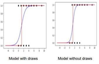
Figure 5: Logistic Regression Model
Decision Trees
A decision tree stands as one of the most straightforward and intuitive methods in automated learning, relying on the divide-and-conquer paradigm. In this structure, an internal node symbolizes a characteristic or attribute, a branch signifies a decision rule, and each leaf node represents an outcome. The tree evolves through recursive splitting.
Decision tree implementation involves the selection of significant features. The execution of a decision tree entails the learning of a decision tree classifier, constructing a tree structure where each internal node (non-leaf node) represents a quality test:
![]()
Here, Pi represents the probability that an arbitrary vector in D belongs to label i [12].
Evaluation Metrics
The fundamental gauge of a classifier's efficacy is its accuracy, quantified as the number of accurately predicted examples divided by the total number of examples. While accuracy is the most prevalent metric for classifier assessment, instances exist where accurately predicted elements of one class differ in value from the prediction value of elements in another class. In such cases, accuracy becomes an insufficient performance metric, necessitating a more nuanced analysis. The confusion matrix proves instrumental in defining various metrics tailored to address these scenarios. In a binary problem, four possible cases are considered:
- True Positives (TP): When the classifier predicts a sample as positive, and it indeed is positive.
- False Positives (FP): When the classifier predicts a sample as positive, but it is, in fact, negative.
- True Negatives (TN): When the classifier predicts a sample as negative, and it truly is negative.
- False Negatives (FN): When the classifier predicts a sample as negative, but it is, in reality, positive [1].
This information is succinctly encapsulated in a matrix known as the confusion matrix, as depicted in Figure 4. To assess the effectiveness of the proposed methods, the following metrics were employed.
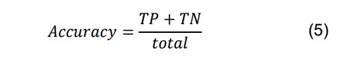
Accuracy: The ratio of correct predictions to the total number of examples.
Precision: The count of correct positive results divided by the total positive results predicted by the classifier.
![]()
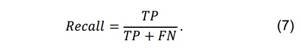
Recall: The count of correct positive results divided by the total positive results.
F1-score: The harmonic mean between precision and recall.
![]()
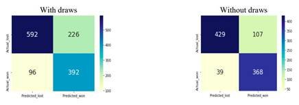
Figure 6: Confusion Matrices
Table 5: Prediction Algorithm Accuracy
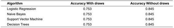
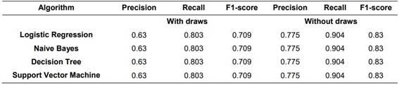
Table 6: Sensitivity, Accuracy, and F1
RESULTS AND DISCUSSION
In Figure 5, a scatter plot illustrates the fit of the regression model (depicted in blue) and the predictions made by the logistic regression model (depicted in red). Key observations include:
- In the prediction model, it is evident that with zero goals, the team tends to lose. However, with one goal, the team has the potential to win a match, but it could also face defeat. Notably, with two or more goals, the team consistently secures a victory.
- Noteworthy changes appear in the logistic regression curve when excluding draws. A more abrupt transition from 0 to 1 is observed compared to the logistic regression curve that considers ties. This discrepancy arises because the likelihood for the logistic regression model, in cases of zero and one goal scored, tends to be closer to zero, while for cases of two or more goals, it tends to be closer to one.
Based on the confusion matrices presented in Figure 6, the accuracy performance without draws reaches 84%, while the inclusion of draws results in 74%, representing the best-case scenarios. Table 5 provides a comparative analysis of accuracy achieved with different algorithms, considering and excluding ties.
Table 6 offers a comprehensive comparison of the four classifier algorithms, along with key classification performance indicators such as precision, recall, and F1 score.
CONCLUSIONS
An extensive analysis of soccer results spanning from 2012 to March 2020 in the Mexican league was conducted, involving 2612 matches before the onset of the pandemic. The study employed four classifier algorithms to predict winning or losing outcomes based on the number of goals scored by a team, achieving comparable accuracy across all algorithms in the best-case scenarios.
The alignment in results is rationalized through the lens of probability. Examining the distribution of goals in Figure 1, without considering draws, the accumulated error amounts to 18.1% in the worst-case scenario—predicting defeat when it is victory and vice versa—resulting in an accuracy of 81.9%. Introducing draws increases the error to 26.9%, with accuracy decreasing to 73.1%. Interestingly, for this specific case, the accuracy remains consistent regardless of the machine learning algorithm employed, with the added observation that there are no instances of 8 goals in the dataset.
Excluding draws enhances accuracy by treating the problem as separable, thereby improving upon the results reported in [5]. Since the prediction task involves only wins and losses, the Softmax Regression model algorithm, suited for multi-class problems, was not utilized.
For future endeavors, the inclusion of additional features could enrich the predictive capacity for soccer match outcomes.
BIBLIOGRAPHICAL REFERENCES
1. Buchdahl, J. (2003). Fixed odds sports betting: statistical forecasting and risk management. High Stakes Publisher, London.
2. Rahman, A. (2020). A deep learning framework for football match prediction. SN Applied Sciences, Vol. 2, No. 165.
3. Behravan, I., Razavi, S. (2020). A novel machine learning method for estimating football players’ value in the transfer market. Soft Computing, Vol. 25, pp. 2499–2511. DOI: 10.1007/s00500-020-05319-3.
4. Domínguez, J., López, B., Mihaylova, P. Georgieva, P. (2019). Incremental learning for football match outcomes prediction. Iberian Conference on Pattern Recognition and Imagine Analysis, pp. 217–228. DOI: 10.1007/978-3-030- 31321-0_19.
5. Igual, L., Seguí, S. (2017). Introduction to data science, a python approach to concepts, techniques and applications. Springer.
6. Scikit learn (2011). Scikit learn developers (BSD License). Support vector machines.
7. Scikit learn (2011). Scikit learn developers (BSD License). Decision trees.
8. Scikit learn (2011). Scikit learn developers (BSD License). Naive Bayes.
9. Paper, D., (2020). Scikit-learn classifier tuning from complex training sets. Hands-on Scikit-Learn for Machine Learning Applications, pp. 165–188. DOI: 10.1007/978-1-4842-5373-1_6. 10. Singh, P. (2019). Machine learning with PySpark, with natural language processing and recommender systems. Second Edition, Apress.
11. Nelli, F. (2018). Python data analytics, with pandas, numpy and matplotlib. Second Edition, Apress.
12. Abdullah, K, Folorunso, S., Solanke, O., Sodimu, S. (2018). A predictive model for tweet sentiment analysis and classification. Annals. Computer Science Series. Vol. 16, No. 2.